3D timelapse from Landsat

Originally posted on 2021-05-04
Last updated 2021-07-02

The purpose of this page is to demonstrate how to make a 3D timelapse animation from Landsat imagery. This code is a bit confusing and hacks together many different workflows. Slowly over time I hope to improve this code.

1 Setup your project

First load the following libraries:

# LANDSAT MOSAICS 
library(mapedit)
library(rgee)
library(sf)

# GAP FILL TIMESERIES
library(stars)
library(forecast)

# RAYSHADER 
library(raster)
library(rayshader)

# ANIMATION
library(gifski)

# PARALLEL 
library(future)
library(future.apply)

Then connect to GEE, more info on connecting your Earth Engine credentials can be found here: https://r-spatial.github.io/rgee/reference/ee_Initialize.html.

rgee::ee_Initialize(email = "", drive = T)

Define your area of interest as an sf polygon. In the commented code below, I use the mapedit package to digitize an aoi, then I save it locally to reproduce the workflow later on. The polygon is then loaded to Earth Engine. There are many ways to do this step.

Pro tip #1: Keep the polygon simple, ideally just a rectangle. Pro tip #2: The larger the polygon, the slower the workflow, start small!

# aoi <- mapedit::editMap() #create AOI
project_name <- "klini_lg" #unique name for the project
# write_sf(aoi, paste0(project_name,".gpkg")) #write aoi locally
aoi <- read_sf(paste0(project_name,".gpkg")) #read from local
aoi_ee <- rgee::sf_as_ee(aoi)$geometry() # convert aoi to earth engine object
Map$centerObject(aoi_ee) #centre map to aoi
Map$addLayer(aoi_ee) #plot aoi from earth engine

Here we set up the project with key variables for the rest of the script. Most are intuitive, but I’ve added some comments to help explain.

resolution <- 30 # Imagery and DEM resolution in m
cloud <- 10 # Landsat metadata cloud cover threshold 
monthStart <- 7 # filter months included in mosaics. 
monthEnd <- 9 # filter months included in mosaics.
yearStart <- 1985 # filter year included in mosaics.
yearEnd <- 2020 # filter year included in mosaics.
yearWindow <- 2 # if 0 mosaics are for 1 year, if 1 then for +- 1 year
yearInterval <- 1 # if 1 then mosaic every year, if 10 then every 10 years. 
years <- seq(yearStart, yearEnd, yearInterval)
cloudBuffer <- 3000 # cloud buffer distance in m
gdrive <- "E:/Google Drive/" # location of google drive locally for files to sync

outfolder_name <- paste( #this is the folder where ALL data will be stored
  project_name,
  resolution, 
  cloud,
  monthStart,
  monthEnd,
  yearStart,
  yearEnd,
  yearInterval,
  yearWindow,
  cloudBuffer,
  sep = "_"
)

2 RGEE

The goal of using Google Earth Engine is to quickly make annual cloud-free mosaics and clip them to our area of interest. The script assumes that you use “Backup and Sync” from Google to automatically sync your Google Drive to your desktop. There are many ways to do this step, this is just one way!

2.1 Landsat functions

# Function to scale Surface Reflectance values
srScale = function(img) {
  img$addBands(img$select(c(
    'blue', 'green', 'red', 'nir', 'swir1', 'swir2'
  ))$multiply(0.0001))$addBands(img$select(c('tir'))$multiply(0.1))$select(
    c('blue_1','green_1','red_1','nir_1','swir1_1','swir2_1','tir_1'),
    c('blue', 'green', 'red', 'nir', 'swir1', 'swir2', 'tir')
  )
}

# Function to remove saturated values
radiometric = function(img) {
  blue = img$select('blue')$eq(2)
  blueAdd = img$select('blue')$subtract(blue)
  green = img$select('green')$eq(2)
  greenAdd = img$select('green')$subtract(green)
  red = img$select('red')$eq(2)
  redAdd = img$select('red')$subtract(red)
  img$addBands(blueAdd)$addBands(greenAdd)$addBands(redAdd)$select(
    c('blue_1', 'green_1', 'red_1', 'nir', 'swir1', 'swir2', 'tir'),ST_NAMES)
}

# Function to apply cloud mask and buffer based on NDCI.
cloudMask = function(img) {
  temp  = img$addBands(img$select('tir')$unitScale(240, 270))
  temp  = temp$addBands(temp$normalizedDifference(c('tir_1', 'swir2'))$rename('ndci'))
  temp  = temp$addBands(temp$select('ndci')$lte(0.4)$rename('ndciT'))
  mask  = temp$select('ndciT')$fastDistanceTransform(51, 'pixels', 'squared_euclidean')$
    sqrt()$multiply(ee$Image$pixelArea()$sqrt())$gt(cloudBuffer)
  img$updateMask(mask)
}

2.2 SR collections

# Load collections
L4SR1 <- ee$ImageCollection('LANDSAT/LT04/C01/T1_SR')
L5SR1 <- ee$ImageCollection('LANDSAT/LT05/C01/T1_SR')
L7SR1v1 <- ee$ImageCollection('LANDSAT/LE07/C01/T1_SR')$
  filterDate('1999-01-01', '2003-01-01')
L7SR1v2 <- ee$ImageCollection('LANDSAT/LE07/C01/T1_SR')$
  filterDate('2012-01-01', '2013-01-01')
L8SR1 <- ee$ImageCollection('LANDSAT/LC08/C01/T1_SR')

# Load bands
LT_BANDS <- c('B1', 'B2', 'B3', 'B4', 'B5', 'B7', 'B6')
LE_BANDS <- c('B1', 'B2', 'B3', 'B4', 'B5', 'B7', 'B6')
LC_BANDS <- c('B2', 'B3', 'B4', 'B5', 'B6', 'B7', 'B10')
ST_NAMES <- c('blue', 'green', 'red', 'nir', 'swir1', 'swir2', 'tir')

# Merge collections and pre-process images
col = L4SR1$select(LT_BANDS, ST_NAMES)$merge(
      L5SR1$select(LT_BANDS, ST_NAMES))$merge(
      L7SR1v1$select(LE_BANDS, ST_NAMES))$merge(
      L7SR1v2$select(LE_BANDS, ST_NAMES))$merge(
      L8SR1$select(LC_BANDS, ST_NAMES))$
  filterBounds(aoi_ee)$filterMetadata('CLOUD_COVER', 'less_than', cloud)$
  filter(ee$Filter$calendarRange(yearStart, yearEnd, "year"))$
  filter(ee$Filter$calendarRange(monthStart, monthEnd, "month"))$
  map(srScale)$
  map(radiometric)$
  map(cloudMask)

# Set Viz params, for visualization and export
vizParams <-
  list(bands = c("swir1", "nir", "red"),
       min = 0,
       max = 0.4)

2.3 Download mosaics

# Loop all years
out <- lapply(years, function(year) {
  print(year)
  
  # Filter Landsat collection to range of years
  col_yr <- col$filter(ee$Filter$calendarRange(year - yearWindow,
                                               year + yearWindow,
                                               "year"))
  # Median Pixel Value
  col_yr_median <- col_yr$median()
  
  # Apply the vizParams to the image
  col_yr_median_rgb <- do.call(col_yr_median$visualize, vizParams)
  
  # Export
  task <- ee$batch$Export$image(
    image = col_yr_median_rgb,
    description = paste0(project_name, "_LS_", year),
    config = list(
      scale = resolution,
      maxPixels = 1.0E13,
      crs = col$first()$projection()$crs()$getInfo(),
      driveFolder = outfolder_name,
      region = aoi_ee
      )
    )
  task$start()
  return(year)
  })

2.4 Download DEM

SRTM is only available above 60°S and below 60°N. If you are wanting to run this outside of the DEM domain, please modify the code to use another dataset.

mydem <- ee$Image("USGS/SRTMGL1_003")
task <- ee$batch$Export$image(
  image = mydem,
  description = paste0(project_name, "_DEM_SRTM"),
  config = list(
    scale = resolution,
    maxPixels = 1.0E13,
    crs = col$first()$projection()$crs()$getInfo(),
    driveFolder = outfolder_name,
    region = aoi_ee
    )
  )

3 Wait 10ish min

WAITING GAME for files to sync locally. There are ways around this with ee_as_raster, but that is not part of this tutorial.

4 Interpolate missing data

We interpolate missing data using the forecast package.

4.1 Inspect tifs

# LIST OF LANDSAT FILES
files_LS <- list.files(paste0(gdrive, outfolder_name), 
                       full.names = T,
                       pattern = "_LS_")

# REDIMENSION THE ENTIRE LIST TO MAKE A PLOT
rgb_LS <- read_stars(files_LS) %>% 
  st_rgb() %>% 
  st_redimension() 

rgb_LS <- rgb_LS %>% 
  st_set_dimensions(3, as.character(years))

rgb_LS %>% plot()

In the figure above, we see black spots. These are no data pixels.

4.2 Impute missing data

# Create output directory 
dir.create(paste0(gdrive,outfolder_name,"/gap_fill"))

# Make a list of the images to interpolate
files_LS <-list.files(paste0(gdrive, outfolder_name),
             full.names = T,
             pattern = "_LS_")

# Define impute function
my_func_ma <- function(vals) {
  vals[vals==0] <- NA
  if(sum(is.na(vals))<25){
    return(as.numeric(forecast::na.interp(vals)))
    }else{
      return(vals)}}

# One band at a time, stack all images of the timeseries and impute. 
slow_impute <- function(band_no){
  
  # READ STACK PER BAND
  band_stack <- read_stars(files_LS)[,,,band_no, drop = T] %>%
    st_redimension() 
  write_stars(band_stack, paste0(gdrive,outfolder_name,"/gap_fill/band",band_no,"_raw.tif"))
  # SMOOTH STACK
  band_stack_ma <- st_apply(band_stack,
                            MARGIN = c("x", "y"),
                            FUN = my_func_ma) %>%
    st_set_dimensions(which = 1,
                      values = as.character(years),
                      names = "year")
  # WRITE OUTPUT
  write_stars(band_stack_ma, paste0(gdrive,outfolder_name,"/gap_fill/band",band_no,"_smooth.tif"))
  return(band_no)}

# RUN THIS IN PARALLEL
plan(multicore)
bands <- 1:3
band_test <- future_lapply(bands, slow_impute)

4.3 Combine into RGB images

# list of the three raster stacks (1 per band) that have been imputed
f <- list.files(paste0(gdrive,outfolder_name,"/gap_fill/"), pattern = "_smooth.tif", full.names = T)

bands <- 1:length(years)

plan(multisession)

# for each band (i.e. year) join into RGB and write
rgb_creator <- function(j){
  i <- read_stars(f[1])[,,,j, drop = T]
  names(i) <- "swir1"
  i$nir <- read_stars(f[2])[,,,j,drop = T]
  i$red <- read_stars(f[3])[,,,j,drop = T]
  i <- i %>% st_redimension()
  write_stars(i, paste0(gdrive,outfolder_name,"/gap_fill/",years[j],"_final.tif"))
  return(j)}

# Run in par
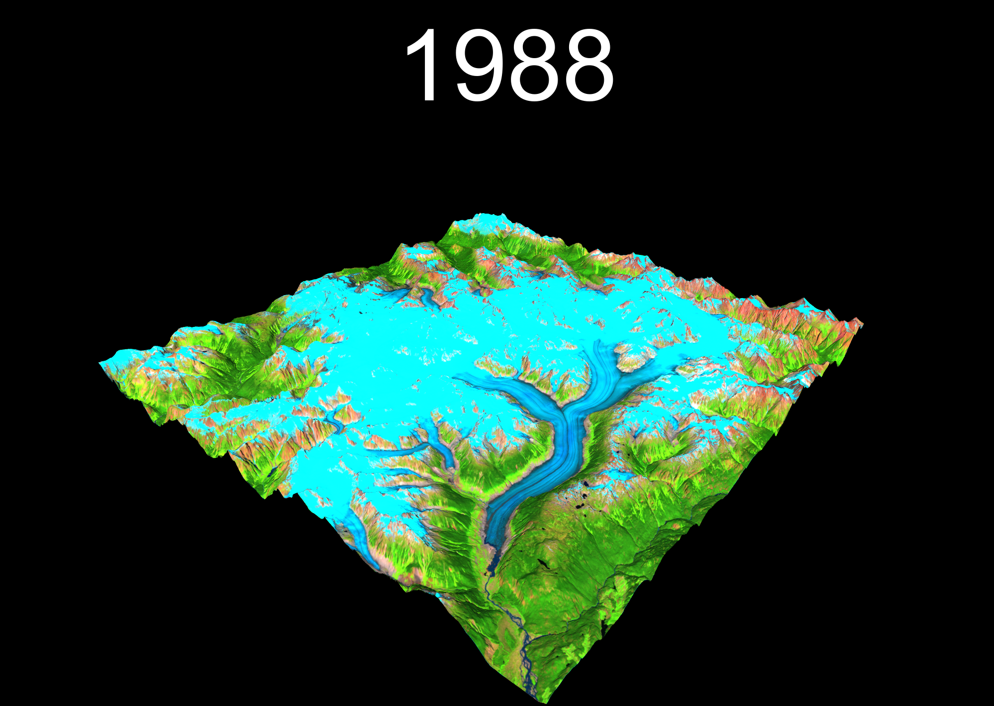
band_test <- future_lapply(bands, rgb_creator)

5 I can rayshade and so can you!

You might need to tinker with the settings to get the best view of your site. Section title inspired from: https://wcmbishop.github.io/rayshader-demo/

dir.create(paste0(gdrive,outfolder_name,"/rayshader_out/"), showWarnings = F)

# LIST LANDSAT FILES 
files_LS <- list.files(paste0(gdrive, outfolder_name,"/gap_fill/"),
                       full.names = T,
                       pattern = "_final.tif")

# LIST DEM FILE
files_DEM <- list.files(paste0(gdrive, outfolder_name),
                        full.names = T,
                        pattern = "_DEM_")

# LOAD DEM 
dem <- raster::raster(files_DEM)
dem_matrix = rayshader::raster_to_matrix(dem, verbose = F)

# LOOP RAYSHADER FOR ALL YEARS

lapply(years, function(year){
  
  img <- raster::stack(files_LS[grep(paste0(year,"_final.tif"), files_LS)])
  
  names(img) = c("r", "g", "b")
  
  img_r = rayshader::raster_to_matrix(img$r, verbose = F)
  img_g = rayshader::raster_to_matrix(img$g, verbose = F)
  img_b = rayshader::raster_to_matrix(img$b, verbose = F)
  
  
  img_array = array(0, dim = c(nrow(img_r), ncol(img_r), 3))
  
  img_array[, , 1] = img_r / 255
  img_array[, , 2] = img_g / 255
  img_array[, , 3] = img_b / 255
  
  img_array = aperm(img_array, c(2, 1, 3))

  temp <- plot_3d(
    img_array,
    dem_matrix,
    windowsize = c(2000,2000),
    zscale = 20, # bigger is flatter
    baseshape = "rectangle",
    solid = TRUE,
    soliddepth = "auto",
    solidcolor = "black",
    solidlinecolor = "black",
    shadow = F,
    theta = 40, # SOUTH = 180
    phi = 30, # NADIR = 90
    fov = 60, #100 = fish-eye
    zoom = 0.8, # small = close
    background = "black"
  )

render_snapshot(
  filename = paste0(gdrive,outfolder_name,"/rayshader_out/",year,".png"),
  title_text = year,
  title_bar_color = "black",
  title_size = 2000*0.1,
  title_color = "white",
  title_position = "north",
  title_bar_alpha = 1
)

rgl::rgl.close()
})

6 I can gifski and so can you!

6.1 In 3D

The gifski package is crazy fast, especially compared to magick..

# Make an output file
dir.create(paste0(gdrive,outfolder_name,"/gif_out/"))

# List of 3D png's
png_files <- list.files(paste0(gdrive,outfolder_name,"/rayshader_out/"), full.names = T)

# Out gif
gif_file <- paste0(paste0(gdrive,outfolder_name,"/animation3d.gif"))

# Animate
gifski(png_files, gif_file,
       width = ncol(png::readPNG(png_files[1])),
       height = nrow(png::readPNG(png_files[1])),
       delay = 0.1,
       loop = TRUE,
       progress = TRUE)

6.2 Or keep it 2D

dir.create(paste0(gdrive,outfolder_name,"/2Dtemp/"))

# List tifs
tif_files <- list.files(paste0(gdrive,outfolder_name,"/gap_fill/"), full.names = T, pattern = "final")

# Write png from tif
plan(multisession)
png_files <- future_lapply(years, function(year){
  out_name <- paste0(gdrive,outfolder_name,"/2Dtemp/", year, "v2.png")
  png(filename = out_name, width = 2000, height = 2000)
  read_stars(paste0(gdrive,outfolder_name,"/gap_fill/",year,"_final.tif")) %>% 
    plot(main = "", rgb = 1:3) 
  dev.off()
  return(out_name)})

# Animate 
gif_file <- paste0(paste0(gdrive,outfolder_name,"/animation2d.gif"))
gifski(unlist(png_files), gif_file,
       width = ncol(png::readPNG(unlist(png_files)[1])),
       height = nrow(png::readPNG(unlist(png_files)[1])),
       delay = 0.1,
       loop = TRUE,
       progress = TRUE)