Originally posted on 2021-05-12 Last updated 2021-07-02

This is a short little project that is in development to make river profiles quickly from the Freshwater Atlas in R. More details can be found here: https://github.com/bcgov/bc-fwa-river-profiles.

The goal of the project is to have a series of R functions where you can simply type the name of a river, and the line work is taken from the freshwater atlas, via the bcdata package, and the DEM is taken from the bcmaps package.

There is quite a bit of functionality missing, but the gist is there for now!

1 Setup project

library(bcdata)
library(tidyverse)
library(ggrepel)
library(stars)
library(sf)
library(bcmaps)

1.1 River names (spelling!)

# Main stem river
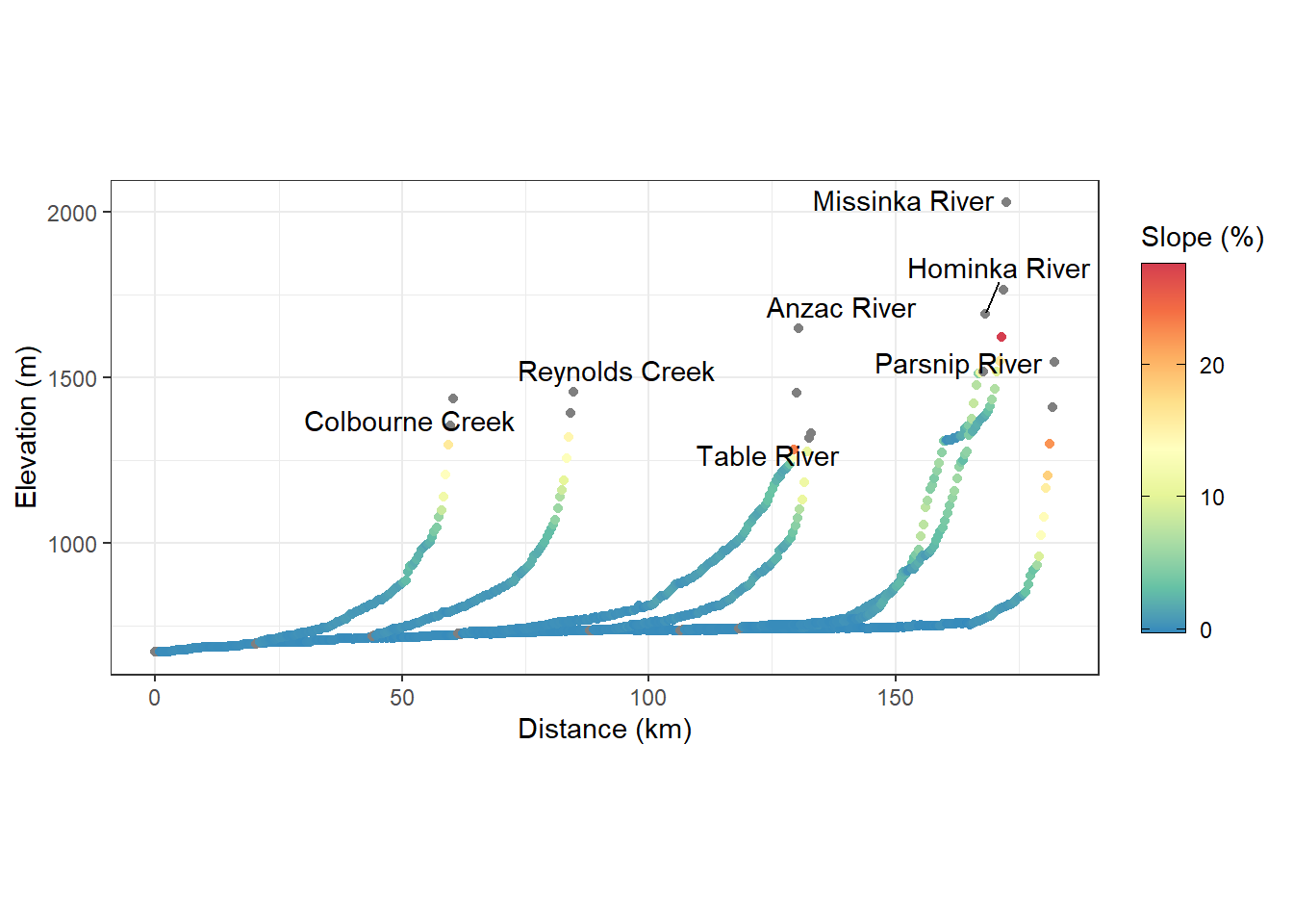
name_ws <- "Parsnip River"

# Tributaries
name_tribs <- c("Anzac River","Hominka River", "Table River", 
                "Missinka River", "Reynolds Creek", "Colbourne Creek")

# How many points per km?
pt_per_km <- 2

# How many points ahead/behind used to calculate slope? 
slp_window_plus_min <- 2

2 Define functions

2.1 Main stem function

fwa_river_profile <- function(
  rivername = "Bowron River",
  pt_per_km = 1,
  check_tiles = T){
  
  # FRESHWATER ATLAS
  
  # Get River Polygons
  my_river <- bcdc_query_geodata("freshwater-atlas-rivers") %>%
    filter(GNIS_NAME_1 == rivername) %>%
    collect()
  
  # Get Unique Code
  my_river_code <- unique(my_river$FWA_WATERSHED_CODE)
  
  # Get Stream Network (lines)
  my_stream_network <- bcdc_query_geodata("freshwater-atlas-stream-network") %>%
    filter(FWA_WATERSHED_CODE == my_river_code) %>%
    collect()
  
  # GET MAINSTEM ONLY
  my_stream_network <-
    my_stream_network %>%
    filter(BLUE_LINE_KEY == unique(my_stream_network$WATERSHED_KEY)) %>% st_as_sf()
  
  # Combine River Segments
  my_stream_network <- st_cast(st_line_merge(
    st_union(st_cast(my_stream_network, "MULTILINESTRING"))), "LINESTRING") %>% st_zm()
  
  # SAMPLE ELEVATION AT POINTS
  
  # GET DEM
  dem <- cded_stars(my_stream_network, check_tiles = check_tiles)
  
  # Make Sample Points
  my_points <- my_stream_network %>%
    st_line_sample(density = units::set_units(pt_per_km, 1/km)) %>%
    st_cast("POINT") %>%
    st_as_sf() %>%
    st_transform(st_crs(dem))
  
  # Extract DEM Values at Points
  my_points_dem <- dem %>%
    st_extract(my_points)  %>%
    mutate(dist_seg_m = replace_na(as.numeric(st_distance(x, lag(x), by_element = TRUE)),0),
           dist_tot_m = cumsum(dist_seg_m),
           id = row_number(),
           river_name = rivername)
  
  return(my_points_dem)
}

2.2 Tributary function

fwa_trib_profile <- function(
  tribname = "Haggen Creek", 
  pt_per_km = 0.5, 
  check_tiles = F, 
  ref = prof_main){
  
  dat_trib <- fwa_river_profile(rivername = tribname, pt_per_km = pt_per_km, check_tiles = check_tiles)
  
  offset <- prof_main %>% 
    mutate(dist = st_distance(., dat_trib %>% filter(elevation == min(dat_trib$elevation)))) %>% 
    arrange(dist) %>% 
    filter(row_number() == 1) %>% 
    select(dist_tot_m)
  
  dat_trib <- dat_trib %>% 
    mutate(dist_tot_m_offset = dist_tot_m + offset$dist_tot_m)
  
  return(dat_trib)
}

3 Run the functions

prof_main <- fwa_river_profile(rivername = name_ws, 
                                   pt_per_km = pt_per_km, 
                                   check_tiles = F)
    
prof_trib <- do.call(bind_rows, lapply(name_tribs, function(name){
  print(name)
  fwa_trib_profile(tribname = name, 
                   pt_per_km = pt_per_km, 
                   check_tiles = F)}))

## [1] "Anzac River"
## [1] "Hominka River"
## [1] "Table River"
## [1] "Missinka River"
## [1] "Reynolds Creek"
## [1] "Colbourne Creek"

4 Add slope

prof_main <- prof_main %>% 
  group_by(river_name) %>% 
  mutate(slope = (
    (lag(elevation,slp_window_plus_min)-lead(elevation,slp_window_plus_min))/
    (lag(dist_tot_m,slp_window_plus_min)-lead(dist_tot_m,slp_window_plus_min)))*100) 

prof_trib <- prof_trib %>% 
  group_by(river_name) %>% 
  mutate(slope = (
    (lag(elevation,slp_window_plus_min)-lead(elevation,slp_window_plus_min))/
    (lag(dist_tot_m,slp_window_plus_min)-lead(dist_tot_m,slp_window_plus_min)))*100)

5 Plot results

prof_trib %>% 
  ggplot() + 
    geom_point(data = prof_main, aes(dist_tot_m/1000, elevation, color = slope), show.legend = T) + 
    geom_point(data = prof_trib, aes(dist_tot_m_offset/1000, elevation, color = slope), show.legend = T) + 
    geom_text_repel(data = prof_main %>%
                             filter(elevation == max(elevation)),
                           aes(dist_tot_m/1000, elevation, label = river_name)) +
    geom_text_repel(data = prof_trib %>%
                             group_by(river_name) %>%
                             filter(elevation == max(elevation)),
                           aes(dist_tot_m_offset/1000, elevation, label = river_name)) +
    scale_color_gradientn(colours = rev(RColorBrewer::brewer.pal(9, "Spectral")), 
                          guide = guide_colourbar(barheight = 10, frame.colour = "black", ticks.colour = "black")) +
    labs(x = "Distance (km)", y = "Elevation (m)", color = "Slope (%)") + 
    theme_bw() +
    theme(aspect.ratio = 0.5)

River profiles in BC